Spark Processing¶

Overview¶

Apache Spark transforms raw VQE simulation results into structured ML feature tables. The processing is batch-oriented and incremental - only new data since the last run is processed.

System Design | Airflow Orchestration

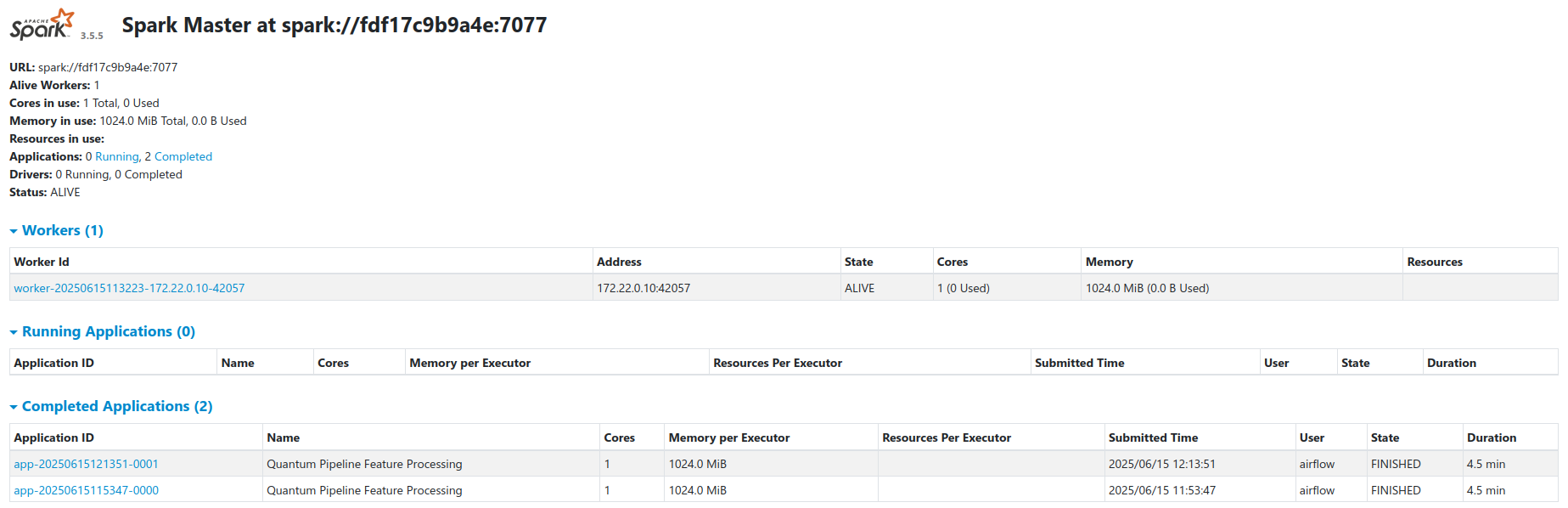
Cluster Architecture¶

The cluster runs in standalone master-worker mode via a custom Spark Docker image (docker/Dockerfile.spark). See the Spark documentation for general cluster configuration.

Node	Role	Resources
`spark-master`	Coordinator	Default (no explicit limits)
`spark-worker`	Executor	1 core, 1 GB RAM (`docker-compose.yaml`)

The thesis compose file (docker-compose.thesis.yaml) increases the worker to 2 cores and 4 GB RAM with explicit resource limits.

Workers register with the master at spark://spark-master:7077
Airflow submits jobs via the SparkSubmitOperator
Workers access MinIO directly through the S3A filesystem connector
Spark Web UI is available at port 8080 on the master node

Spark Web UI showing the master node with registered workers and completed applications — Figure 1. Spark Web UI displaying the master node with registered workers and job execution history.

Feature Engineering Pipeline¶

A 6-step workflow transforms raw VQE results into nine feature tables. Each run is incremental.

Step 1: Create Spark Session¶

A SparkSession is initialized with S3A (MinIO connectivity), Iceberg catalog integration, and adaptive query execution. The configuration is defined in DEFAULT_CONFIG at the top of the processing script.

spark = (
    SparkSession.builder
    .appName(config.get('APP_NAME'))
    .master(config.get('SPARK_MASTER'))
    .config('spark.sql.extensions',
            'org.apache.iceberg.spark.extensions.IcebergSparkSessionExtensions')
    .config('spark.sql.catalog.quantum_catalog',
            'org.apache.iceberg.spark.SparkCatalog')
    .config('spark.sql.catalog.quantum_catalog.type', 'hadoop')
    .config('spark.sql.catalog.quantum_catalog.warehouse',
            config.get('S3_WAREHOUSE'))
    .config('spark.hadoop.fs.s3a.impl',
            'org.apache.hadoop.fs.s3a.S3AFileSystem')
    .config('spark.hadoop.fs.s3a.endpoint', config.get('S3_ENDPOINT'))
    .config('spark.hadoop.fs.s3a.path.style.access', 'true')
    .config('spark.sql.adaptive.enabled', 'true')
    .config('spark.sql.shuffle.partitions', '200')
    .getOrCreate()
)

Default S3 paths from DEFAULT_CONFIG:

Experiment bucket: s3a://local-vqe-results/experiments/
Feature warehouse: s3a://local-features/warehouse/

Step 2: Initialize Iceberg Metadata¶

The job reads or initializes the Iceberg metadata catalog. If this is the first run, the catalog and database are created. On subsequent runs, existing metadata is loaded to determine which data has already been processed.

def list_available_topics(spark, bucket_path):
    """List available topics from the storage."""
    fs = spark._jvm.org.apache.hadoop.fs.FileSystem.get(
        spark._jvm.java.net.URI.create(bucket_path),
        spark._jsc.hadoopConfiguration()
    )
    path = spark._jvm.org.apache.hadoop.fs.Path(bucket_path)
    if fs.exists(path) and fs.isDirectory(path):
        return [f.getPath().getName() for f in fs.listStatus(path)
                if f.isDirectory()]
    return []

Step 3: Filter New Data¶

New records are identified by joining against existing Iceberg table keys. A marker-column approach is used instead of left_anti to handle edge cases.

def identify_new_records(spark, new_data_df, table_name, key_columns):
    """Identify records not yet present in the target Iceberg table."""
    if not spark.catalog.tableExists(
            f'quantum_catalog.quantum_features.{table_name}'):
        return new_data_df

    existing_keys = spark.sql(
        f'SELECT DISTINCT {", ".join(key_columns)} '
        f'FROM quantum_catalog.quantum_features.{table_name}'
    )

    if existing_keys.isEmpty():
        return new_data_df

    # Marker-column join to find only new records
    new_with_marker = (new_data_df.select(*key_columns).distinct()
                       .withColumn('is_new', lit(1)))
    existing_with_marker = existing_keys.withColumn('exists', lit(1))
    joined = new_with_marker.join(existing_with_marker,
                                  on=key_columns, how='left')
    new_keys = joined.filter(col('exists').isNull()).select(*key_columns)
    return new_data_df.join(new_keys, on=key_columns, how='inner')

Step 4: Extract Features¶

Raw VQE data is transformed into nine specialized feature tables. The transform_quantum_data function flattens nested Avro fields and adds metadata columns (experiment_id, processing_timestamp, processing_date, processing_batch_id).

def transform_quantum_data(df):
    """Transform raw VQE data into specialized feature tables."""
    base_df = add_metadata_columns(df, 'quantum_base_processing')
    # Flatten nested Avro fields into a wide DataFrame, then
    # select columns for each feature table:
    return {
        'molecules': df_molecule,
        'ansatz_info': df_ansatz,
        'performance_metrics': df_metrics,
        'vqe_results': df_vqe,
        'initial_parameters': df_initial_parameters,
        'optimal_parameters': df_optimal_parameters,
        'vqe_iterations': df_iterations,
        'iteration_parameters': df_iteration_parameters,
        'hamiltonian_terms': df_hamiltonian,
    }

See docker/airflow/scripts/quantum_incremental_processing.py for the full implementation of each extraction.

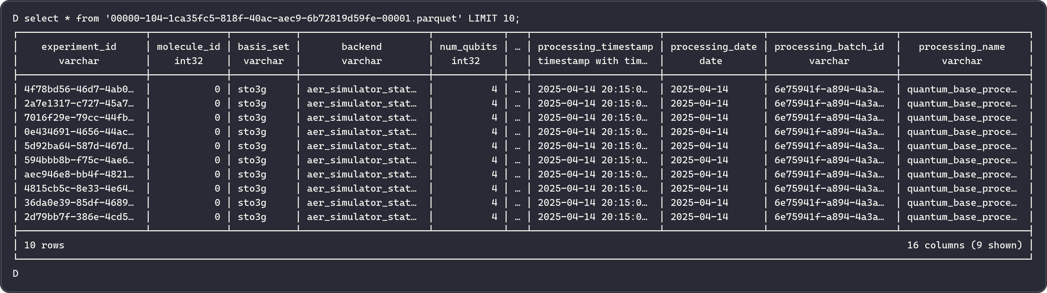
Step 5: Write Parquet to MinIO¶

Feature data is written as Parquet through the Iceberg table API. New tables are created on first run; subsequent runs append only new records.

def process_incremental_data(spark, new_data_df, table_name, key_columns,
                             partition_columns=None):
    """Write new data to an Iceberg table, creating it if necessary."""
    table_path = f'quantum_catalog.quantum_features.{table_name}'

    if not spark.catalog.tableExists(table_path):
        writer = new_data_df.write.format('iceberg') \
            .option('write-format', 'parquet')
        if partition_columns:
            writer = writer.partitionBy(*partition_columns)
        writer.mode('overwrite').saveAsTable(table_path)
    else:
        truly_new = identify_new_records(spark, new_data_df,
                                         table_name, key_columns)
        if truly_new.count() > 0:
            truly_new.write.format('iceberg') \
                .option('write-format', 'parquet') \
                .mode('append') \
                .saveAsTable(table_path)

Step 6: Update Iceberg Snapshots¶

After writing, a tagged Iceberg snapshot records the processing batch ID for time-travel queries. Initial writes use v_{batch_id} tags; incremental appends use v_incr_{batch_id}.

snapshot_id = spark.sql(
    f'SELECT snapshot_id '
    f'FROM quantum_catalog.quantum_features.{table_name}.snapshots '
    f'ORDER BY committed_at DESC LIMIT 1'
).collect()[0][0]

version_tag = f'v_{processing_batch_id}'
spark.sql(f"""
    ALTER TABLE quantum_catalog.quantum_features.{table_name}
    CREATE TAG {version_tag} AS OF VERSION {snapshot_id}
""")

Feature Tables¶

Nine tables stored as Iceberg-managed Parquet files in MinIO under quantum_catalog.quantum_features.

Preview of processed Parquet feature data showing structured columns and values — Figure 2. Preview of processed feature data in Parquet format, queried with DuckDB.

1. `molecules`¶

Molecular structure information for each simulated molecule.

Column	Type	Description
`experiment_id`	string	Unique experiment identifier
`molecule_id`	int	Molecule identifier
`atom_symbols`	array<string>	Chemical symbols (e.g., ["H", "H"])
`coordinates`	array<array<double>>	3D atomic coordinates
`multiplicity`	int	Spin multiplicity
`charge`	int	Molecular charge
`coordinate_units`	string	Units (angstrom or bohr)
`atomic_masses`	array<double>	Atomic masses (amu)

Partitioned by: processing_date

2. `ansatz_info`¶

Quantum circuit ansatz configurations used in each experiment.

Column	Type	Description
`experiment_id`	string	Unique experiment identifier
`molecule_id`	int	Molecule identifier
`basis_set`	string	Basis set (e.g., `sto3g`, `cc-pvdz`)
`ansatz`	string	QASM3 circuit representation
`ansatz_reps`	int	Number of ansatz repetitions

Partitioned by: processing_date, basis_set

3. `performance_metrics`¶

Execution timing and performance data for each simulation.

Column	Type	Description
`experiment_id`	string	Unique experiment identifier
`molecule_id`	int	Molecule identifier
`basis_set`	string	Basis set
`hamiltonian_time`	double	Hamiltonian construction time (seconds)
`mapping_time`	double	Fermionic-to-qubit mapping time (seconds)
`vqe_time`	double	VQE optimization time (seconds)
`total_time`	double	Total simulation time (seconds)
`minimization_time`	double	Optimizer execution time (seconds)
`computed_total_time`	double	Sum of `hamiltonian_time` + `mapping_time` + `vqe_time`

Partitioned by: processing_date, basis_set

4. `vqe_results`¶

Core VQE optimization results including the minimum energy found.

Column	Type	Description
`experiment_id`	string	Unique experiment identifier
`molecule_id`	int	Molecule identifier
`basis_set`	string	Basis set
`backend`	string	Qiskit backend (e.g., `aer_simulator`)
`num_qubits`	int	Number of qubits in the circuit
`optimizer`	string	Optimizer algorithm (e.g., `L-BFGS-B`, `COBYLA`)
`noise_backend`	string	Noise model used (if any)
`default_shots`	int	Number of shots per circuit execution
`ansatz_reps`	int	Number of ansatz repetitions
`minimum_energy`	double	Ground state energy estimate (Hartree)
`maxcv`	double	Maximum constraint violation
`total_iterations`	int	Number of optimizer iterations

Partitioned by: processing_date, basis_set, backend

5. `initial_parameters`¶

Starting variational parameters for each experiment.

Column	Type	Description
`parameter_id`	string	Unique parameter identifier
`experiment_id`	string	Experiment identifier
`molecule_id`	int	Molecule identifier
`basis_set`	string	Basis set
`backend`	string	Qiskit backend
`num_qubits`	int	Number of qubits
`parameter_index`	int	Parameter position in the circuit
`initial_parameter_value`	double	Starting parameter value

Partitioned by: processing_date, basis_set

6. `optimal_parameters`¶

Optimized variational parameters after VQE convergence.

Column	Type	Description
`parameter_id`	string	Unique parameter identifier
`experiment_id`	string	Experiment identifier
`molecule_id`	int	Molecule identifier
`basis_set`	string	Basis set
`backend`	string	Qiskit backend
`num_qubits`	int	Number of qubits
`parameter_index`	int	Parameter position in the circuit
`optimal_parameter_value`	double	Optimized parameter value

Partitioned by: processing_date, basis_set

7. `vqe_iterations`¶

Per-iteration optimization data recording the energy at each step.

Column	Type	Description
`iteration_id`	string	Unique iteration identifier
`experiment_id`	string	Experiment identifier
`molecule_id`	int	Molecule identifier
`basis_set`	string	Basis set
`backend`	string	Qiskit backend
`num_qubits`	int	Number of qubits
`iteration_step`	int	Iteration number
`iteration_energy`	double	Energy at this step (Hartree)
`energy_std_dev`	double	Standard deviation of measurement

Partitioned by: processing_date, basis_set, backend

8. `iteration_parameters`¶

Parameter values at each optimizer iteration, enabling convergence analysis.

Column	Type	Description
`parameter_id`	string	Unique parameter identifier
`iteration_id`	string	Iteration identifier
`experiment_id`	string	Experiment identifier
`molecule_id`	int	Molecule identifier
`basis_set`	string	Basis set
`backend`	string	Qiskit backend
`num_qubits`	int	Number of qubits
`iteration_step`	int	Iteration number
`parameter_value`	double	Parameter value at this iteration

Partitioned by: processing_date, basis_set

9. `hamiltonian_terms`¶

Hamiltonian Pauli operator terms and their complex coefficients.

Column	Type	Description
`term_id`	string	Unique term identifier
`experiment_id`	string	Experiment identifier
`molecule_id`	int	Molecule identifier
`basis_set`	string	Basis set
`backend`	string	Qiskit backend
`term_label`	string	Pauli string (e.g., "XYZI", "IIZZ")
`coeff_real`	double	Real part of the coefficient
`coeff_imag`	double	Imaginary part of the coefficient

Partitioned by: processing_date, basis_set, backend

Incremental Processing¶

Spark uses Iceberg metadata to identify and process only new records on each run.

How It Works¶

List current files - Spark enumerates all Avro files in the MinIO experiments bucket.
Check Iceberg snapshots - If an Iceberg snapshot exists from a previous run, the system retrieves the set of already-processed file paths.
Compute delta - New files are identified as the difference between current files and previously processed files.
Process delta only - Only the new files are read, transformed, and appended to the feature tables.
Update snapshot - A new Iceberg snapshot is created, recording the current set of processed files.

System Design - Full architecture overview
Airflow Orchestration - Spark job scheduling
Iceberg Storage - Table format and snapshots
Kafka Streaming - Raw data ingestion

Spark Processing¶

Overview¶

Cluster Architecture¶

Feature Engineering Pipeline¶

Step 1: Create Spark Session¶

Step 2: Initialize Iceberg Metadata¶

Step 3: Filter New Data¶

Step 4: Extract Features¶

Step 5: Write Parquet to MinIO¶

Step 6: Update Iceberg Snapshots¶

Feature Tables¶

1. molecules¶

2. ansatz_info¶

3. performance_metrics¶

4. vqe_results¶

5. initial_parameters¶

6. optimal_parameters¶

7. vqe_iterations¶

8. iteration_parameters¶

9. hamiltonian_terms¶

Incremental Processing¶

How It Works¶

Related Documentation¶

References¶

1. `molecules`¶

2. `ansatz_info`¶

3. `performance_metrics`¶

4. `vqe_results`¶

5. `initial_parameters`¶

6. `optimal_parameters`¶

7. `vqe_iterations`¶

8. `iteration_parameters`¶

9. `hamiltonian_terms`¶