System Design Documentation¶

Overview¶

This chapter presents the architecture of the system designed for simulating and processing Variational Quantum Eigensolver (VQE) algorithm results.

It consists of the following key components:

Simulation module
Apache Kafka message broker
MinIO storage system
Apache Airflow orchestrator
Apache Spark processing engine (master-worker configuration with one worker)

Each component communicates with the others through a Docker container network, ensuring isolation, consistency, and the ability to scale independently. The architecture is based on the microservices pattern.

Architecture Principles¶

The system follows several key architectural principles:

Separation of Concerns: Each component has a well-defined responsibility
Loose Coupling: Components communicate through well-defined interfaces
Scalability: Horizontal scaling capabilities for compute-intensive tasks
Data Versioning: Immutable data with schema evolution support
Incremental Processing: Only process new data to optimize resources
Observability: Comprehensive monitoring and metrics collection

1. Quantum Simulation Module¶

Overview¶

The main simulation module prepares data for simulation and executes VQE simulations using the Qiskit Aer simulator. The system was designed with the capability to integrate with real quantum computers via IBM Quantum, but due to access costs, only the simulator is extensively tested and used in this project.

The VQE algorithm is monitored during execution - data is collected from each optimizer iteration, execution times for individual stages, and information about the molecule and the basis set used.

Each simulation module container also exports system metrics (CPU and RAM usage) to Prometheus PushGateway, enabling resource monitoring in a containerized environment.

VQE Execution Pipeline¶

sequenceDiagram
    participant User
    participant VQERunner
    participant QiskitAer
    participant Monitor
    participant Prometheus
    participant Kafka

    User->>VQERunner: Start VQE Simulation
    VQERunner->>VQERunner: Load Molecule
    VQERunner->>VQERunner: Build Hamiltonian
    Note over VQERunner: Track hamiltonian_time

    VQERunner->>VQERunner: Map to Qubits
    Note over VQERunner: Track mapping_time

    VQERunner->>Monitor: Start Performance Monitoring
    Monitor->>Prometheus: Export System Metrics

    VQERunner->>QiskitAer: Execute VQE
    loop Each Optimizer Iteration
        QiskitAer->>QiskitAer: Evaluate Cost Function
        QiskitAer->>Monitor: Log Iteration Data
        Monitor->>Monitor: Store Parameters & Energy
    end
    Note over QiskitAer: Track vqe_time

    QiskitAer->>VQERunner: Return Optimization Result
    VQERunner->>VQERunner: Aggregate Results
    Note over VQERunner: Calculate total_time

    VQERunner->>Kafka: Publish VQEDecoratedResult
    Monitor->>Prometheus: Export Final Metrics
    VQERunner->>User: Simulation Complete

Hold "Alt" / "Option" to enable pan & zoom

Data Collection During Execution¶

All collected data are aggregated into a single result object, which size depends on the problem complexity and the number of algorithm iterations.

The monitoring system collects:

Iteration Data: Parameters, energy values, and standard deviation for each optimizer step
Timing Information:
- hamiltonian_time: Time to construct the molecular Hamiltonian
- mapping_time: Time to map fermionic operators to qubit operators
- vqe_time: VQE optimization execution time
- total_time: Total simulation time
Molecule Information: Atomic symbols, coordinates, charge, multiplicity, basis set
System Metrics: CPU usage, memory consumption, container resource utilization

VQEDecoratedResult Interface¶

The implementation uses Apache Avro as the data serialization format.

VQEDecoratedResultInterface class is responsible for serialization, deserialization, and managing the data schema in the schema registry.

This separation of responsibilities ensures data format consistency between different system components. Long term planned is migration to a more readable and less cluttered Pydantic structure.

class VQEDecoratedResultInterface(AvroInterfaceBase[VQEDecoratedResult]):
    def __init__(self, registry):
        super().__init__(registry)
        self.result_interface = VQEResultInterface(self.registry)
        self.molecule_interface = MoleculeInfoInterface(self.registry)
        self.schema_name = 'vqe_decorated_result'

    @property
    def schema(self) -> dict[str, Any]:
        try:
            return self.registry.get_schema(self.schema_name)
        except FileNotFoundError:
            schema = {
                'type': 'record',
                'name': 'VQEDecoratedResult',
                'fields': [
                    {'name': 'vqe_result', 'type': self.result_interface.schema},
                    {'name': 'molecule', 'type': self.molecule_interface.schema},
                    {'name': 'basis_set', 'type': 'string'},
                    {'name': 'hamiltonian_time', 'type': 'double'},
                    {'name': 'mapping_time', 'type': 'double'},
                    {'name': 'vqe_time', 'type': 'double'},
                    {'name': 'total_time', 'type': 'double'},
                    {'name': 'molecule_id', 'type': 'int'},
                ],
            }
            dict_schema = deepcopy(schema)
            self.registry.save_schema(self.schema_name, schema)
            return dict_schema

    def serialize(self, obj: VQEDecoratedResult) -> dict[str, Any]:
        return {
            'vqe_result': self.result_interface.serialize(obj.vqe_result),
            'molecule': self.molecule_interface.serialize(obj.molecule),
            'basis_set': obj.basis_set,
            'hamiltonian_time': float(obj.hamiltonian_time),
            'mapping_time': float(obj.mapping_time),
            'vqe_time': float(obj.vqe_time),
            'total_time': float(obj.total_time),
            'molecule_id': obj.molecule_id,
        }

    def deserialize(self, data: dict[str, Any]) -> VQEDecoratedResult:
        return VQEDecoratedResult(
            vqe_result=self.result_interface.deserialize(data['vqe_result']),  # Simulation results - including each iteration
            molecule=self.molecule_interface.deserialize(data['molecule']),    # Information about simulated molecule
            basis_set=data['basis_set'],                                       # Basis set - determines simulation accuracy
            hamiltonian_time=float64(data['hamiltonian_time']),                # Time to build Hamiltonian operator
            mapping_time=float64(data['mapping_time']),                        # Mapping time
            vqe_time=float64(data['vqe_time']),                                # VQE algorithm simulation time
            total_time=float64(data['total_time']),                            # Total simulation time
            molecule_id=int(data['molecule_id']),                              # Molecule identifier
        )

Schema Structure Breakdown¶

Nested Schema Architecture

The VQEDecoratedResult schema uses a compositional design pattern, where complex types are built from simpler nested schemas.

Top-Level Schema: VQEDecoratedResult¶

Field	Type	Description
`vqe_result`	VQEResult (nested)	Complete VQE optimization results
`molecule`	MoleculeInfo (nested)	Molecular structure information
`basis_set`	string	Basis set used (e.g., `sto3g`, `cc-pvdz`)
`hamiltonian_time`	double	Hamiltonian construction time (seconds)
`mapping_time`	double	Fermionic-to-qubit mapping time (seconds)
`vqe_time`	double	VQE optimization execution time (seconds)
`total_time`	double	Total end-to-end execution time (seconds)
`molecule_id`	int	Unique molecule identifier

VQEResult Schema¶

Field	Type	Description
`initial_data`	VQEInitialData (nested)	Initial configuration and parameters
`iteration_list`	array<VQEProcess>	Complete iteration history
`minimum`	double	Minimum energy found (Hartree)
`optimal_parameters`	array<double>	Optimal circuit parameters
`maxcv`	double (nullable)	Maximum constraint violation
`minimization_time`	double	Optimizer execution time (seconds)

VQEInitialData Schema¶

Field	Type	Description
`backend`	string	Qiskit backend name (e.g., "aer_simulator")
`num_qubits`	int	Number of qubits in circuit
`hamiltonian`	array<HamiltonianTerm>	Pauli operator terms with coefficients
`num_parameters`	int	Number of variational parameters
`initial_parameters`	array<double>	Starting parameter values
`optimizer`	string	Optimizer name (e.g., "L-BFGS-B")
`ansatz`	string	QASM3 representation of circuit
`ansatz_reps`	int	Number of ansatz repetitions
`noise_backend`	string	Noise model configuration
`default_shots`	int	Number of measurement shots

VQEProcess Schema (Iteration Data)¶

Field	Type	Description
`iteration`	int	Iteration number
`parameters`	array<double>	Parameter values at this iteration
`result`	double	Energy value (Hartree)
`std`	double	Standard deviation of measurement

MoleculeInfo Schema¶

Field	Type	Description
`symbols`	array<string>	Atomic symbols (e.g., ["H", "H"])
`coords`	array<array<double>>	3D coordinates (Angstrom or Bohr)
`multiplicity`	int	Spin multiplicity
`charge`	int	Total molecular charge
`units`	string	Coordinate units ("angstrom" or "bohr")
`masses`	array<double> (nullable)	Atomic masses (amu)

HamiltonianTerm Schema¶

Field	Type	Description
`label`	string	Pauli string (e.g., "XYZI", "IIZZ")
`coefficients`	ComplexNumber	Complex coefficient

ComplexNumber Schema¶

Field	Type	Description
`real`	double	Real component
`imaginary`	double	Imaginary component

Serialization Details¶

Type Conversion Strategy

The Avro interface handles automatic conversion between Python/NumPy types and Avro-compatible primitives:

numpy.float64 -> double
numpy.int64 -> long / int
numpy.ndarray -> array<T>
Complex numbers -> {real: double, imaginary: double}

Binary Serialization with Schema Registry¶

After serialization, data is transmitted to Apache Kafka. The serialization process includes:

Schema Registration: Schema is registered with Confluent Schema Registry
Magic Byte Prefix: Binary data starts with 0x00 (Confluent wire format)
Schema ID: 4-byte big-endian schema identifier
Avro Binary Data: Compact binary-encoded payload

def to_avro_bytes(self, obj: T, schema_name: str = 'vqe_decorated_result') -> bytes:
    """Convert object to Avro binary format."""
    schema = self.schema
    parsed_schema = avro.schema.parse(json.dumps(schema))

    writer = DatumWriter(parsed_schema)
    bytes_writer = io.BytesIO()

    # Write Confluent Schema Registry header
    bytes_writer.write(bytes([0]))  # Magic byte
    bytes_writer.write(self.registry.id_cache[schema_name].to_bytes(4, byteorder='big'))

    encoder = BinaryEncoder(bytes_writer)
    writer.write(self.serialize(obj), encoder)
    return bytes_writer.getvalue()

Container Metrics Export¶

Each simulation container exports metrics to Prometheus PushGateway:

graph LR
    QC1[Quantum Container 1] -->|HTTP POST| PG[Prometheus PushGateway]
    QC2[Quantum Container 2] -->|HTTP POST| PG
    QC3[Quantum Container 3] -->|HTTP POST| PG
    PG -->|Scrape| PROM[Prometheus]
    PROM -->|Query| GRAF[Grafana Dashboards]

    style QC1 fill:#c5cae9,color:#1a237e
    style QC2 fill:#c5cae9,color:#1a237e
    style QC3 fill:#c5cae9,color:#1a237e
    style PG fill:#e8f5e9,color:#1b5e20
    style PROM fill:#e8f5e9,color:#1b5e20
    style GRAF fill:#e8f5e9,color:#1b5e20

Hold "Alt" / "Option" to enable pan & zoom

Exported Metrics:

quantum_system_cpu_percent: CPU utilization percentage
quantum_system_memory_percent: Memory utilization percentage
quantum_vqe_total_time: Total VQE execution time
quantum_vqe_minimum_energy: Minimum energy value found
quantum_vqe_iterations_count: Number of optimizer iterations

2. Apache Kafka Integration¶

Schema Registry Automatic Versioning¶

The Schema Registry provides several key capabilities:

Automatic Version Management: Each schema change creates a new version
Compatibility Mode: Currently set to NONE (unrestricted changes in development)
Schema Evolution: Supports adding/removing fields with default values
Centralized Schema Store: Single source of truth for data structures

Schema Compatibility

The system uses NONE compatibility mode in the connector configuration, allowing unrestricted schema evolution. For production, consider BACKWARD or FULL compatibility. See the Confluent Schema Evolution docs for details.

Kafka Configuration Parameters¶

Producer ConfigurationKafka ClusterSchema Registry

@dataclass
class ProducerConfig:
    servers: str          # Kafka bootstrap servers
    topic: str            # Target topic name
    security: SecurityConfig
    retries: int = 3      # Application-level retries
    retry_delay: int = 2  # Delay between retries (seconds)
    kafka_retries: int = 5  # Kafka internal retries
    acks: str = 'all'     # Acknowledgment level
    timeout: int = 10     # Producer timeout (seconds)

Kafka runs in KRaft mode.

kafka:
  image: bitnami/kafka:latest
  environment:
    - KAFKA_CFG_NODE_ID=0
    - KAFKA_CFG_PROCESS_ROLES=controller,broker
    - KAFKA_CFG_CONTROLLER_QUORUM_VOTERS=0@kafka:9093
    - KAFKA_CFG_LISTENERS=PLAINTEXT://kafka:9092,CONTROLLER://:9093,EXTERNAL://0.0.0.0:9094
    - KAFKA_CFG_ADVERTISED_LISTENERS=PLAINTEXT://kafka:9092,EXTERNAL://localhost:9094
    - KAFKA_CFG_LISTENER_SECURITY_PROTOCOL_MAP=CONTROLLER:PLAINTEXT,PLAINTEXT:PLAINTEXT,EXTERNAL:PLAINTEXT
    - KAFKA_CFG_CONTROLLER_LISTENER_NAMES=CONTROLLER
    - KAFKA_CFG_INTER_BROKER_LISTENER_NAME=PLAINTEXT

schema-registry:
  image: confluentinc/cp-schema-registry:7.5.0
  environment:
    SCHEMA_REGISTRY_HOST_NAME: schema-registry
    SCHEMA_REGISTRY_KAFKASTORE_BOOTSTRAP_SERVERS: 'kafka:9092'
    SCHEMA_REGISTRY_LISTENERS: 'http://0.0.0.0:8081'
    SCHEMA_REGISTRY_SCHEMA_COMPATIBILITY_LEVEL: 'none'

Parallel Version Support¶

Allows multiple versions of the simulation module to run in parallel (e.g., when testing new functionality) without the risk of data structure conflicts. Kafka buffers results from multiple parallel simulator instances, ensuring transmission reliability in case of temporary consumer unavailability.

sequenceDiagram
    participant P1 as Producer v1
    participant P2 as Producer v2
    participant K as Kafka
    participant SR as Schema Registry
    participant C as Consumer

    P1->>SR: Register Schema v1
    SR-->>P1: Schema ID: 101

    P2->>SR: Register Schema v2
    SR-->>P2: Schema ID: 102

    par Parallel Production
        P1->>K: Publish to vqe_decorated_result_v1
        P2->>K: Publish to vqe_decorated_result_v2
    end

    C->>K: Subscribe to vqe_decorated_result_.*
    K->>C: Deliver messages from v1
    K->>C: Deliver messages from v2

    Note over C: Consumer handles both versions

Hold "Alt" / "Option" to enable pan & zoom

Use Cases:

A/B Testing: Run different algorithm configurations simultaneously
Blue-Green Deployments: Deploy new version without stopping old one
Canary Releases: Gradually roll out schema changes
Development/Production Isolation: Separate topics for different environments

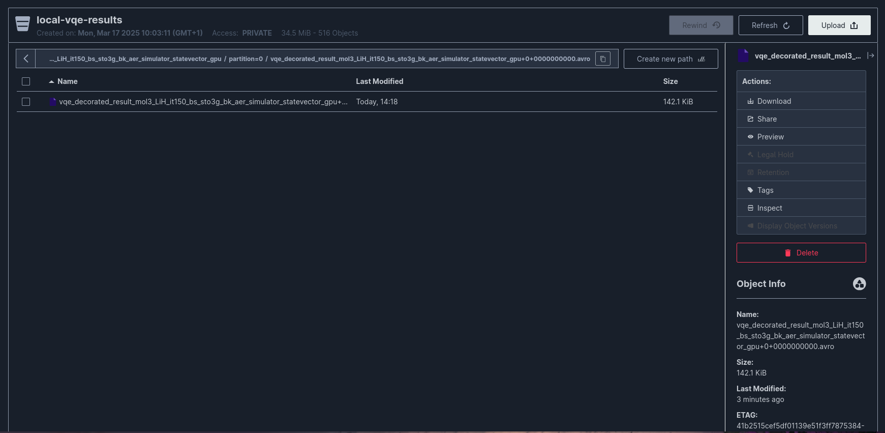
3. MinIO Integration¶

S3-Compatible Object Storage¶

For persistent data storage, the system uses MinIO - an object storage compatible with the Amazon S3 API. Data is automatically transferred from Kafka to MinIO using the Kafka Connect S3 Sink connector.

graph LR
    K[Kafka Topics] -->|Stream| KC[Kafka Connect]
    KC <-->|Validate| SR[Schema Registry]
    KC -->|S3 PutObject| MINIO[MinIO<br/>local-vqe-results]

    style K fill:#ffe082,color:#000
    style KC fill:#ffe082,color:#000
    style SR fill:#ffe082,color:#000
    style MINIO fill:#b39ddb,color:#311b92

Hold "Alt" / "Option" to enable pan & zoom

Kafka Connect S3 Sink Connector Configuration¶

The following configuration defines how data is stored, the serialization format, and connection parameters to MinIO:

{
  "name": "minio-sink",
  "config": {
    "connector.class": "io.confluent.connect.s3.S3SinkConnector",
    "tasks.max": "1",

    "topics.regex": "vqe_decorated_result_.*",
    "refresh.topics.enabled": "true",

    "topics.dir": "experiments",
    "directory.delim": "/",

    "s3.bucket.name": "local-vqe-results",
    "store.url": "http://minio:9000",
    "s3.region": "us-east-1",
    "s3.path.style.access": "true",
    "s3.access.key.id": "admin",
    "s3.secret.access.key": "admin123",
    "s3.part.size": "5242880",
    "s3.retry.backoff.ms": "1000",

    "flush.size": "1",
    "schema.compatibility": "NONE",
    "storage.class": "io.confluent.connect.s3.storage.S3Storage",
    "format.class": "io.confluent.connect.s3.format.avro.AvroFormat",

    "key.converter": "io.confluent.connect.avro.AvroConverter",
    "value.converter": "io.confluent.connect.avro.AvroConverter",
    "key.converter.schema.registry.url": "http://schema-registry:8081",
    "value.converter.schema.registry.url": "http://schema-registry:8081",

    "errors.tolerance": "all",
    "errors.log.enable": "true",
    "errors.log.include.messages": "true"
  }
}

Connector Configuration

Key project-specific choices: flush.size: 1 for immediate write-through, schema.compatibility: NONE for unrestricted schema evolution, and s3.path.style.access: true required for MinIO. See the Confluent S3 Sink Connector docs for parameter details.

Directory Structure in MinIO¶

The connector creates the following directory structure:

s3://local-vqe-results/
└── experiments/
    ├── vqe_decorated_result_v1/
    │   ├── partition=0/
    │   │   ├── vqe_decorated_result_v1+0+0000000000.avro
    │   │   ├── vqe_decorated_result_v1+0+0000000001.avro
    │   │   └── vqe_decorated_result_v1+0+0000000002.avro
    │   ├── partition=1/
    │   │   └── vqe_decorated_result_v1+1+0000000000.avro
    │   └── partition=2/
    │       └── vqe_decorated_result_v1+2+0000000000.avro
    └── vqe_decorated_result_v2/
        ├── partition=0/
        │   └── vqe_decorated_result_v2+0+0000000000.avro
        └── partition=1/
            └── vqe_decorated_result_v2+1+0000000000.avro

File Naming Convention:

{topic_name}+{partition}+{start_offset}.avro

Example: vqe_decorated_result_v1+0+0000000000.avro

Topic: vqe_decorated_result_v1
Partition: 0
Start Offset: 0000000000

MinIO browser showing LiH molecule data stored in the object storage — Figure 3. MinIO object storage browser displaying stored VQE results for the LiH molecule.

Data Consistency Guarantees¶

The connector configuration ensures data consistency through:

Feature	Configuration	Guarantee
Exactly-Once Semantics	`enable.idempotence: true` (producer)	No duplicate writes
Durability	`acks: all` (producer)	Data persisted to all replicas
Error Handling	`errors.tolerance: all`	Failed messages logged but processing continues
Schema Validation	Schema Registry integration	Only valid messages written to MinIO

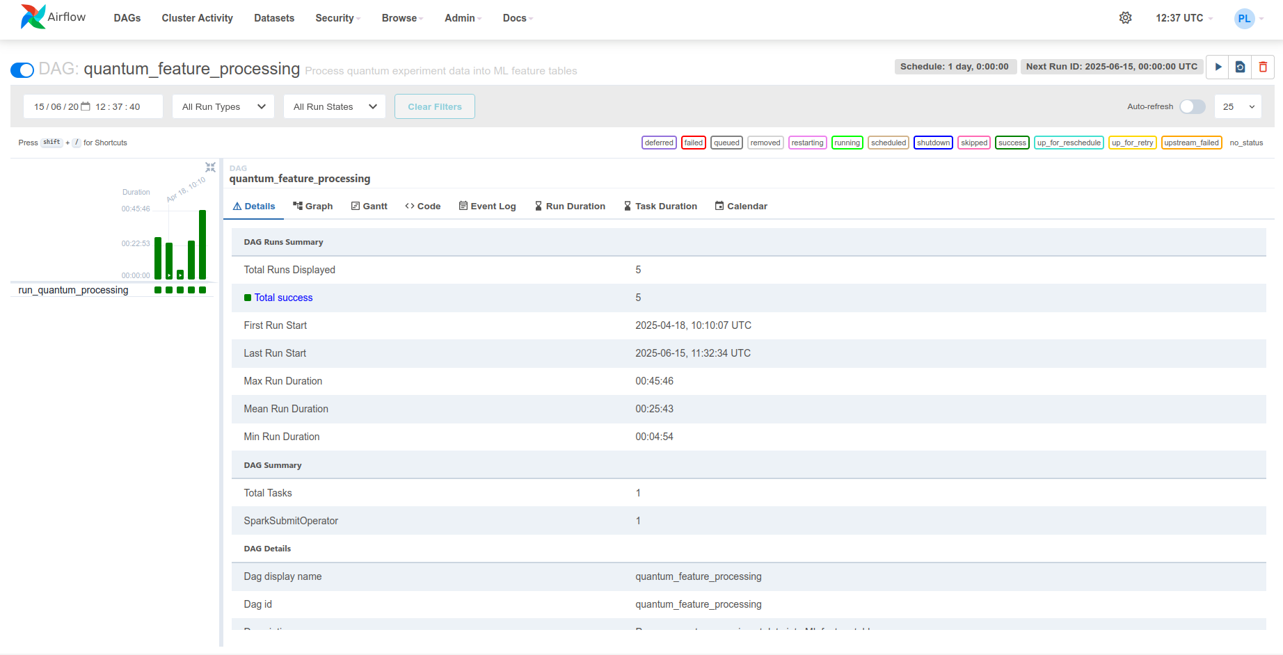
4. Apache Airflow Orchestration¶

Workflow Orchestration¶

Apache Airflow orchestrates the data processing workflow by managing the processing schedule. In this project, Airflow runs a daily incremental processing task (schedule_interval=timedelta(days=1)) that delegates computations to Apache Spark.

graph LR
    subgraph "Airflow"
        DAG["Feature Processing<br/>DAG"]
        VARS["Variables<br/>MinIO credentials · Spark settings"]
        DAG -->|reads| VARS
    end

    SPARK[Spark Cluster]

    subgraph "Storage"
        MINIO[(MinIO<br/>Raw Iceberg tables)]
        ICEBERG[(MinIO<br/>Feature tables)]
    end

    DAG -->|SparkSubmitOperator| SPARK
    SPARK -->|read| MINIO
    SPARK -->|write| ICEBERG

    style DAG fill:#90caf9,color:#0d47a1
    style SPARK fill:#a5d6a7,color:#1b5e20
    style MINIO fill:#ffe082,color:#e65100
    style ICEBERG fill:#ffe082,color:#e65100

Hold "Alt" / "Option" to enable pan & zoom

DAG Definition¶

The DAG (Directed Acyclic Graph) defines the task for processing quantum experiment results into ML features:

with DAG(
    'quantum_feature_processing',
    default_args={**default_args, 'retries': 3, 'retry_delay': timedelta(minutes=20)},
    description='Process quantum experiment data into ML feature tables',
    schedule_interval=timedelta(days=1),
    start_date=datetime(2025, 1, 1),
    catchup=False,
    tags=['quantum', 'ML', 'features', 'processing', 'Apache Spark'],
    on_success_callback=send_success_email,
) as dag:
    quantum_simulation_results_processing = SparkSubmitOperator(
        task_id='run_quantum_processing',
        application='/opt/airflow/dags/scripts/quantum_incremental_processing.py',
        conn_id='spark_default',
        name='quantum_feature_processing',
        conf={
            'spark.master': Variable.get('SPARK_MASTER'),
            'spark.app.name': Variable.get('APP_NAME'),
            'spark.hadoop.fs.s3a.endpoint': Variable.get('S3_ENDPOINT'),
            'spark.hadoop.fs.s3a.access.key': Variable.get('MINIO_ACCESS_KEY'),
            'spark.hadoop.fs.s3a.secret.key': Variable.get('MINIO_SECRET_KEY'),
            'spark.hadoop.fs.s3a.path.style.access': 'true',
            'spark.hadoop.fs.s3a.connection.ssl.enabled': 'false',
            'spark.jars.packages': (
                'org.slf4j:slf4j-api:2.0.17,'
                'commons-codec:commons-codec:1.18.0,'
                'com.google.j2objc:j2objc-annotations:3.0.0,'
                'org.apache.spark:spark-avro_2.12:3.5.5,'
                'org.apache.hadoop:hadoop-aws:3.3.1,'
                'org.apache.hadoop:hadoop-common:3.3.1,'
                'org.apache.iceberg:iceberg-spark-runtime-3.5_2.12:1.4.2'
            ),
        },
        env_vars={
            'MINIO_ACCESS_KEY': Variable.get('MINIO_ACCESS_KEY'),
            'MINIO_SECRET_KEY': Variable.get('MINIO_SECRET_KEY'),
            'S3_ENDPOINT': Variable.get('S3_ENDPOINT'),
            'S3_BUCKET': Variable.get('S3_BUCKET'),
            'S3_WAREHOUSE': Variable.get('S3_WAREHOUSE'),
            'SPARK_MASTER': Variable.get('SPARK_MASTER'),
        },
        verbose=True,
    )

The DAG runs daily with catchup=False (no backfill), retries up to 3 times with 20-minute delays, and sends email notifications on success/failure. For Airflow scheduling and retry configuration details, see the Apache Airflow docs.

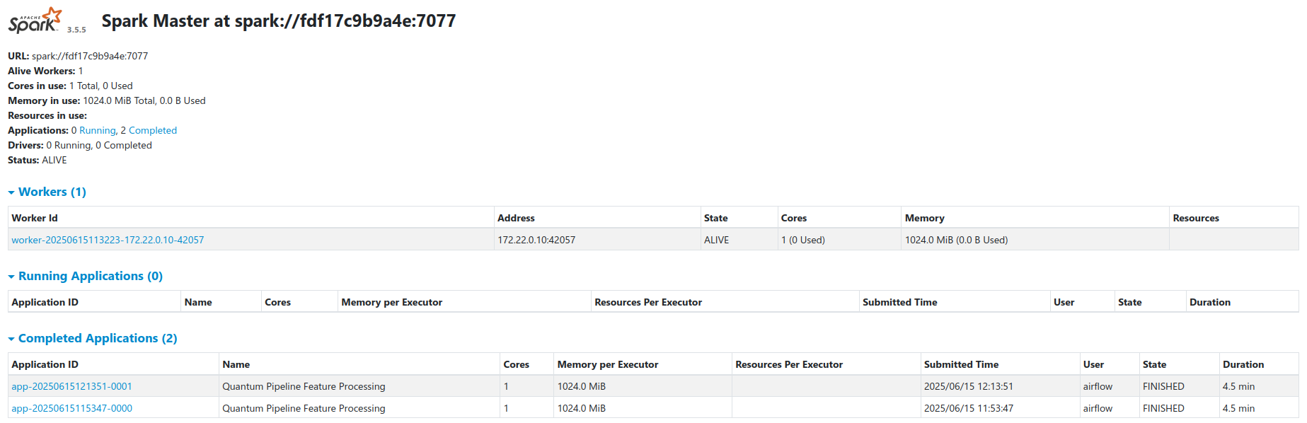
The SparkSubmitOperator delegates to the Spark cluster. All connection parameters (MinIO credentials, Spark master URL, S3 endpoints) are managed through Airflow Variables, initialized from the DEFAULT_CONFIG dict in quantum_incremental_processing.py and environment variables.

Default Configuration Values (from DEFAULT_CONFIG in the processing script):

DEFAULT_CONFIG = {
    'S3_ENDPOINT': 'http://minio:9000',
    'SPARK_MASTER': 'spark://spark-master:7077',
    'S3_BUCKET': 's3a://local-vqe-results/experiments/',
    'S3_WAREHOUSE': 's3a://local-features/warehouse/',
    'APP_NAME': 'Quantum Pipeline Feature Processing',
}

DAG Execution Flow¶

sequenceDiagram
    participant S as Airflow Scheduler
    participant E as Airflow Executor
    participant SSO as SparkSubmitOperator
    participant SM as Spark Master
    participant SW as Spark Workers
    participant M as MinIO
    participant I as Iceberg

    Note over S: Cron: Daily at 00:00
    S->>E: Schedule quantum_feature_processing
    E->>SSO: Execute run_quantum_processing

    SSO->>SSO: Read Airflow Variables
    SSO->>SM: Submit PySpark job

    SM->>SW: Distribute tasks

    par Read Raw Data
        SW->>M: Read Avro files from experiments/
    end

    SW->>SW: Transform to feature tables

    par Write Features
        SW->>I: Write to Iceberg tables
    end

    I->>I: Create snapshot
    I->>M: Persist Parquet files

    SW->>SM: Report completion
    SM->>SSO: Job finished
    SSO->>E: Task success
    E->>S: Update DAG state

    alt Success
        S->>S: Send success email
    else Failure
        S->>S: Retry (up to 3 times)
        S->>S: Send failure email
    end

Hold "Alt" / "Option" to enable pan & zoom

The Airflow web UI is accessible at http://airflow:8084 for monitoring DAG execution, task status, and logs.

Apache Airflow DAG view showing the quantum processing pipeline — Figure 2. Apache Airflow DAG view for the quantum feature processing workflow.

5. Incremental Processing¶

Overview¶

The system implements incremental processing, meaning that only new data since the last run is processed. This eliminates the need to repeatedly process the same results and significantly reduces execution time and computational resource usage.

Apache Iceberg provides a mechanism for tracking the state of processed data through a metadata layer. Iceberg stores information about data snapshots, enabling Spark to efficiently detect which files in MinIO have already been processed and which are new.

graph LR
    RAW[(MinIO<br/>Raw Avro files)]
    META[Iceberg Metadata<br/>Last processed snapshot]

    subgraph "Spark"
        FILTER[Identify new files]
        PROC[Compute features]
        FILTER -->|new files only| PROC
    end

    FEAT[(MinIO<br/>Feature tables)]

    RAW -->|list files| FILTER
    META -->|last snapshot| FILTER
    PROC --> FEAT
    PROC -->|update snapshot| META

    style FILTER fill:#ffe082,color:#000
    style RAW fill:#90caf9,color:#0d47a1
    style FEAT fill:#a5d6a7,color:#1b5e20
    style META fill:#b39ddb,color:#311b92

Hold "Alt" / "Option" to enable pan & zoom

6-Step Processing Workflow¶

The incremental processing workflow consists of the following steps:

Step 1: Create Spark Session with MinIO Configuration¶

def create_spark_session(config=None):
    """Create and configure a Spark session with Iceberg and S3 support."""
    if config is None:
        config = DEFAULT_CONFIG

    validate_environment()

    access_key = os.environ.get('MINIO_ACCESS_KEY')
    secret_key = os.environ.get('MINIO_SECRET_KEY')

    return (
        SparkSession.builder
        .appName(config.get('APP_NAME'))
        .master(config.get('SPARK_MASTER'))
        .config('spark.jars.packages', (
            'org.apache.spark:spark-avro_2.12:3.5.5,'
            'org.apache.hadoop:hadoop-aws:3.3.1,'
            'org.apache.iceberg:iceberg-spark-runtime-3.5_2.12:1.4.2'
        ))
        .config('spark.sql.extensions',
                'org.apache.iceberg.spark.extensions.IcebergSparkSessionExtensions')
        .config('spark.sql.catalog.quantum_catalog',
                'org.apache.iceberg.spark.SparkCatalog')
        .config('spark.sql.catalog.quantum_catalog.type', 'hadoop')
        .config('spark.sql.catalog.quantum_catalog.warehouse',
                config.get('S3_WAREHOUSE'))
        .config('spark.hadoop.fs.s3a.impl',
                'org.apache.hadoop.fs.s3a.S3AFileSystem')
        .config('spark.hadoop.fs.s3a.access.key', access_key)
        .config('spark.hadoop.fs.s3a.secret.key', secret_key)
        .config('spark.hadoop.fs.s3a.endpoint', config.get('S3_ENDPOINT'))
        .config('spark.hadoop.fs.s3a.path.style.access', 'true')
        .config('spark.hadoop.fs.s3a.connection.ssl.enabled', 'false')
        .config('spark.sql.adaptive.enabled', 'true')
        .config('spark.sql.shuffle.partitions', '200')
        .getOrCreate()
    )

The session configures the quantum_catalog Iceberg catalog backed by a Hadoop warehouse on MinIO (s3a://local-features/warehouse/), with adaptive query execution enabled and 200 shuffle partitions.

Step 2: Initialize or Read Iceberg Metadata¶

def list_available_topics(spark, bucket_path):
    """List available topics from the storage."""
    fs = spark._jvm.org.apache.hadoop.fs.FileSystem.get(
        spark._jvm.java.net.URI.create(bucket_path),
        spark._jsc.hadoopConfiguration()
    )

    path = spark._jvm.org.apache.hadoop.fs.Path(bucket_path)

    if fs.exists(path) and fs.isDirectory(path):
        return [f.getPath().getName() for f in fs.listStatus(path) if f.isDirectory()]
    return []

Iceberg Metadata Structure:

s3a://local-features/warehouse/
└── quantum_features/
    ├── vqe_results/
    │   ├── metadata/
    │   │   ├── v1.metadata.json
    │   │   ├── v2.metadata.json
    │   │   ├── snap-1234567890.avro
    │   │   └── snap-1234567891.avro
    │   └── data/
    │       ├── part-00000.parquet
    │       └── part-00001.parquet
    └── vqe_iterations/
        ├── metadata/
        └── data/

Step 3: Filter Data - Select Only New Files¶

def identify_new_records(spark, new_data_df, table_name, key_columns):
    """
    Identifies records in new_data_df that don't exist in the target table.
    Uses DataFrame operations for better performance.
    """
    # If table does not exist, every record is new
    if not spark.catalog.tableExists(f'quantum_catalog.quantum_features.{table_name}'):
        return new_data_df

    # Retrieve existing keys
    existing_keys = spark.sql(
        f'SELECT DISTINCT {", ".join(key_columns)} '
        f'FROM quantum_catalog.quantum_features.{table_name}'
    )

    # If table exists but has no records - return all records
    if existing_keys.isEmpty():
        return new_data_df

    # Anti-join to find new records
    new_with_marker = new_data_df.select(*key_columns).distinct().withColumn('is_new', lit(1))
    existing_with_marker = existing_keys.withColumn('exists', lit(1))

    joined = new_with_marker.join(existing_with_marker, on=key_columns, how='left')
    new_keys = joined.filter(col('exists').isNull()).select(*key_columns)

    # Join back to get full records
    truly_new_data = new_data_df.join(new_keys, on=key_columns, how='inner')

    return truly_new_data

Deduplication Logic:

graph LR
    A[New Data<br/>experiment_id: 1,2,3,4] --> B{Table Exists?}
    B -->|No| C[All Records are New<br/>1,2,3,4]
    B -->|Yes| D[Existing Data<br/>experiment_id: 1,2]
    D --> E[Left Anti-Join]
    A --> E
    E --> F[Truly New Records<br/>experiment_id: 3,4]

    style C fill:#a5d6a7,color:#1b5e20
    style F fill:#a5d6a7,color:#1b5e20

Hold "Alt" / "Option" to enable pan & zoom

Step 4: Process Data - Extract Features¶

def transform_quantum_data(df):
    """Transforms the original quantum data into various feature tables."""
    base_df = add_metadata_columns(df, 'quantum_base_processing')

    # Extract nested fields
    base_df = base_df.select(
        col('experiment_id'),
        col('molecule_id'),
        col('basis_set'),
        col('vqe_result.initial_data').alias('initial_data'),
        col('vqe_result.iteration_list').alias('iteration_list'),
        col('vqe_result.minimum').alias('minimum_energy'),
        # ... more fields
    )

    # Create specialized feature tables
    return {
        'molecules': extract_molecule_features(base_df),
        'vqe_results': extract_vqe_features(base_df),
        'vqe_iterations': extract_iteration_features(base_df),
        'hamiltonian_terms': extract_hamiltonian_features(base_df),
        # ... 9 total feature tables
    }

Feature Table Transformations:

Molecules TableVQE Results TableIterations Table

df_molecule = base_df.select(
    col('experiment_id'),
    col('molecule_id'),
    col('molecule_data.symbols').alias('atom_symbols'),
    col('molecule_data.coords').alias('coordinates'),
    col('molecule_data.multiplicity').alias('multiplicity'),
    col('molecule_data.charge').alias('charge'),
    col('processing_timestamp'),
    col('processing_date'),
)

df_vqe = base_df.select(
    col('experiment_id'),
    col('molecule_id'),
    col('basis_set'),
    col('initial_data.backend').alias('backend'),
    col('initial_data.num_qubits').alias('num_qubits'),
    col('initial_data.optimizer').alias('optimizer'),
    col('minimum_energy'),
    size(col('iteration_list')).alias('total_iterations'),
    col('processing_date'),
)

df_iterations = base_df.select(
    col('experiment_id'),
    explode(col('iteration_list')).alias('iteration'),
).select(
    col('experiment_id'),
    col('iteration.iteration').alias('iteration_step'),
    col('iteration.result').alias('iteration_energy'),
    col('iteration.std').alias('energy_std_dev'),
)

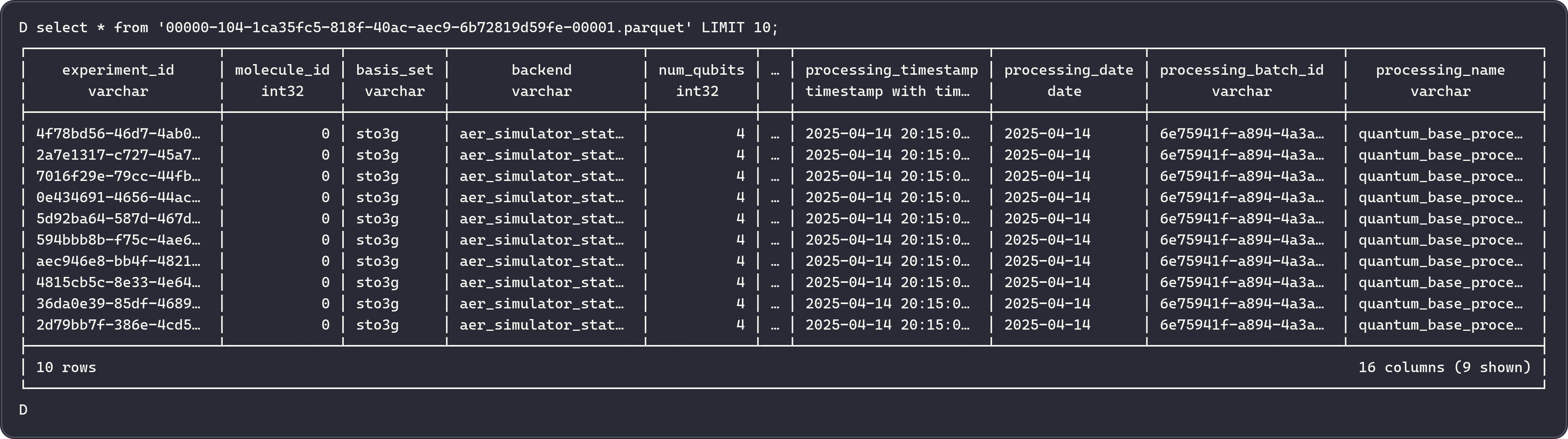
Step 5: Write Processed Data in Parquet Format¶

def process_incremental_data(spark, new_data_df, table_name, key_columns,
                             partition_columns=None, comment=None):
    """Process the data incrementally - only data that wasn't processed yet."""

    # Check if table exists
    table_exists = spark.catalog._jcatalog.tableExists(
        f'quantum_catalog.quantum_features.{table_name}'
    )

    if not table_exists:
        # Create new table
        writer = new_data_df.write.format('iceberg').option('write-format', 'parquet')

        if partition_columns:
            writer = writer.partitionBy(*partition_columns)

        writer.mode('overwrite').saveAsTable(
            f'quantum_catalog.quantum_features.{table_name}'
        )
    else:
        # Append only new records
        truly_new_data = identify_new_records(spark, new_data_df, table_name, key_columns)

        if truly_new_data.count() == 0:
            return None, 0

        truly_new_data.write.format('iceberg') \
            .option('write-format', 'parquet') \
            .mode('append') \
            .saveAsTable(f'quantum_catalog.quantum_features.{table_name}')

    return version_tag, record_count

Data is written in Parquet columnar format via Iceberg.

Step 6: Update Iceberg Metadata - Create New Snapshot¶

# Create a tag for this version of the table
snapshot_id = spark.sql(
    f'SELECT snapshot_id FROM quantum_catalog.quantum_features.{table_name}.snapshots '
    f'ORDER BY committed_at DESC LIMIT 1'
).collect()[0][0]

processing_batch_id = new_data_df.limit(1).collect()[0]['processing_batch_id'].replace('-', '')
version_tag = f'v_{processing_batch_id}'

spark.sql(f"""
    ALTER TABLE quantum_catalog.quantum_features.{table_name}
    CREATE TAG {version_tag} AS OF VERSION {snapshot_id}
""")

Iceberg Snapshot Management:

graph TB
    subgraph "Timeline"
        S1[Snapshot 1<br/>2025-01-10 00:00<br/>Tag: v_initial]
        S2[Snapshot 2<br/>2025-01-11 00:00<br/>Tag: v_incr_abc123]
        S3[Snapshot 3<br/>2025-01-12 00:00<br/>Tag: v_incr_def456]
        S4[Snapshot 4<br/>Current]
    end

    S1 -->|+100 records| S2
    S2 -->|+50 records| S3
    S3 -->|+75 records| S4

    subgraph "Time Travel Queries"
        Q1[SELECT * FROM table<br/>VERSION AS OF v_initial]
        Q2[SELECT * FROM table<br/>TIMESTAMP AS OF '2025-01-11']
        Q3[SELECT * FROM table<br/>FOR SYSTEM_TIME AS OF '2025-01-12']
    end

    Q1 -.->|Returns| S1
    Q2 -.->|Returns| S2
    Q3 -.->|Returns| S3

    style S4 fill:#b39ddb,color:#311b92

Hold "Alt" / "Option" to enable pan & zoom

Time-Travel Queries:

-- Query data as of specific snapshot
SELECT * FROM quantum_catalog.quantum_features.vqe_results
VERSION AS OF 'v_incr_abc123';

-- Query data at specific timestamp
SELECT * FROM quantum_catalog.quantum_features.vqe_results
TIMESTAMP AS OF '2025-01-11 12:00:00';

-- Compare snapshots
SELECT current.*, previous.*
FROM quantum_catalog.quantum_features.vqe_results FOR SYSTEM_VERSION AS OF 12345 AS current
JOIN quantum_catalog.quantum_features.vqe_results FOR SYSTEM_VERSION AS OF 12344 AS previous
ON current.experiment_id = previous.experiment_id
WHERE current.minimum_energy != previous.minimum_energy;

Feature Tables Schema¶

The system creates 9 specialized feature tables:

1. molecules2. ansatz_info3. performance_metrics4. vqe_results5. initial_parameters6. optimal_parameters7. vqe_iterations8. iteration_parameters9. hamiltonian_terms

Purpose: Molecular structure information

Column	Type	Description
experiment_id	string	Unique experiment identifier
molecule_id	int	Molecule identifier
atom_symbols	array<string>	Chemical symbols
coordinates	array<array<double>>	3D coordinates
multiplicity	int	Spin multiplicity
charge	int	Molecular charge
coordinate_units	string	Units (angstrom/bohr)
atomic_masses	array<double>	Atomic masses

Partitioning: processing_date

Purpose: Quantum circuit ansatz configurations

Column	Type	Description
experiment_id	string	Unique experiment identifier
molecule_id	int	Molecule identifier
basis_set	string	Basis set (e.g., `sto3g`)
ansatz	string	QASM3 circuit representation
ansatz_reps	int	Number of repetitions

Partitioning: processing_date, basis_set

Purpose: Execution timing and performance

Column	Type	Description
experiment_id	string	Unique experiment identifier
molecule_id	int	Molecule identifier
basis_set	string	Basis set
hamiltonian_time	double	Hamiltonian build time (s)
mapping_time	double	Mapping time (s)
vqe_time	double	VQE execution time (s)
total_time	double	Total time (s)
minimization_time	double	Optimizer time (s)

Partitioning: processing_date, basis_set

Purpose: VQE optimization results

Column	Type	Description
experiment_id	string	Unique experiment identifier
molecule_id	int	Molecule identifier
basis_set	string	Basis set
backend	string	Qiskit backend
num_qubits	int	Number of qubits
optimizer	string	Optimizer algorithm
minimum_energy	double	Ground state energy (Ha)
total_iterations	int	Number of iterations

Partitioning: processing_date, basis_set, backend

Purpose: Initial variational parameters

Column	Type	Description
parameter_id	string	Unique parameter identifier
experiment_id	string	Experiment identifier
molecule_id	int	Molecule identifier
parameter_index	int	Parameter position
initial_parameter_value	double	Initial value

Partitioning: processing_date, basis_set

Purpose: Optimized variational parameters

Column	Type	Description
parameter_id	string	Unique parameter identifier
experiment_id	string	Experiment identifier
molecule_id	int	Molecule identifier
parameter_index	int	Parameter position
optimal_parameter_value	double	Optimized value

Partitioning: processing_date, basis_set

Purpose: Per-iteration optimization data

Column	Type	Description
iteration_id	string	Unique iteration identifier
experiment_id	string	Experiment identifier
molecule_id	int	Molecule identifier
iteration_step	int	Iteration number
iteration_energy	double	Energy at this step (Ha)
energy_std_dev	double	Standard deviation

Partitioning: processing_date, basis_set, backend

Purpose: Parameters at each iteration

Column	Type	Description
parameter_id	string	Unique parameter identifier
iteration_id	string	Iteration identifier
experiment_id	string	Experiment identifier
iteration_step	int	Iteration number
parameter_value	double	Parameter value

Partitioning: processing_date, basis_set

Purpose: Hamiltonian Pauli operator terms

Column	Type	Description
term_id	string	Unique term identifier
experiment_id	string	Experiment identifier
molecule_id	int	Molecule identifier
term_label	string	Pauli string (e.g., "XYZI")
coeff_real	double	Real coefficient
coeff_imag	double	Imaginary coefficient

Partitioning: processing_date, basis_set, backend

Apache Spark master UI showing the quantum feature processing job — Figure 4. Apache Spark master interface during quantum feature processing execution.

Preview of Parquet feature table data — Figure 5. Preview of a processed feature table stored in Parquet format.

Efficient Filtering of Processed Files¶

The incremental processing system uses several optimization strategies:

1. Partition Pruning¶

# Only scan partitions for today
df = spark.read.format('iceberg') \
    .load('quantum_catalog.quantum_features.vqe_results') \
    .filter(col('processing_date') == current_date())

2. Predicate Pushdown¶

-- Filter pushed to storage layer
SELECT * FROM quantum_catalog.quantum_features.vqe_results
WHERE basis_set = 'sto3g' AND minimum_energy < -1.0;

3. Metadata-Only Queries¶

-- No data file reads required
SELECT COUNT(*) FROM quantum_catalog.quantum_features.vqe_results;

SELECT MIN(minimum_energy), MAX(minimum_energy)
FROM quantum_catalog.quantum_features.vqe_results;

4. File-Level Deduplication¶

Iceberg tracks individual data files, avoiding re-reading already processed files:

# Iceberg automatically skips files already in the table
new_files = set(current_files) - set(processed_files_in_snapshot)

Metadata Tracking Table¶

The system maintains a metadata table to track all processing runs:

CREATE TABLE IF NOT EXISTS quantum_catalog.quantum_features.processing_metadata (
    processing_batch_id STRING,
    processing_name STRING,
    processing_timestamp TIMESTAMP,
    processing_date DATE,
    table_names ARRAY<STRING>,
    table_versions ARRAY<STRING>,
    record_counts ARRAY<BIGINT>,
    source_data_info STRING
) USING iceberg

Deployment Architecture¶

Docker Compose Services¶

The complete platform is deployed using Docker Compose with the following services:

services:
  # Data Streaming Layer - KRaft mode
  kafka:
    image: bitnami/kafka:latest

  schema-registry:
    image: confluentinc/cp-schema-registry:7.5.0
    depends_on:
      - kafka

  kafka-connect:
    image: confluentinc/cp-kafka-connect:7.5.0
    depends_on:
      - kafka
      - schema-registry
      - minio

  # Storage Layer
  minio:
    image: minio/minio:latest

  # Processing Layer
  spark-master:
    image: straightchlorine/quantum-pipeline:spark

  spark-worker:
    image: straightchlorine/quantum-pipeline:spark
    depends_on:
      - spark-master

  # Orchestration Layer
  postgres:
    image: postgres:14

  airflow-webserver:
    image: straightchlorine/quantum-pipeline:airflow
    depends_on:
      - postgres

  airflow-scheduler:
    image: straightchlorine/quantum-pipeline:airflow
    depends_on:
      - postgres

  # Quantum Simulation
  quantum-pipeline:
    image: straightchlorine/quantum-pipeline:latest
    depends_on:
      - kafka
      - schema-registry

Monitoring and Observability¶

The system exports metrics to Prometheus via PushGateway (VQE execution metrics, resource utilization). Grafana dashboards are accessible at http://grafana:3000 for VQE execution monitoring, data pipeline health. For details on the monitoring stack configuration, see the Monitoring section.